From data to predictions and a loss function

One dot product makes one prediction

Put observations in the rows of a data matrix $X$. A weight vector $w$ tells us how strongly each feature contributes. The matrix product computes all the predictions:

If $X$ has $m$ rows and $n$ columns, $w$ has $n$ entries and $\hat y$ has $m$ entries—one prediction per observation.

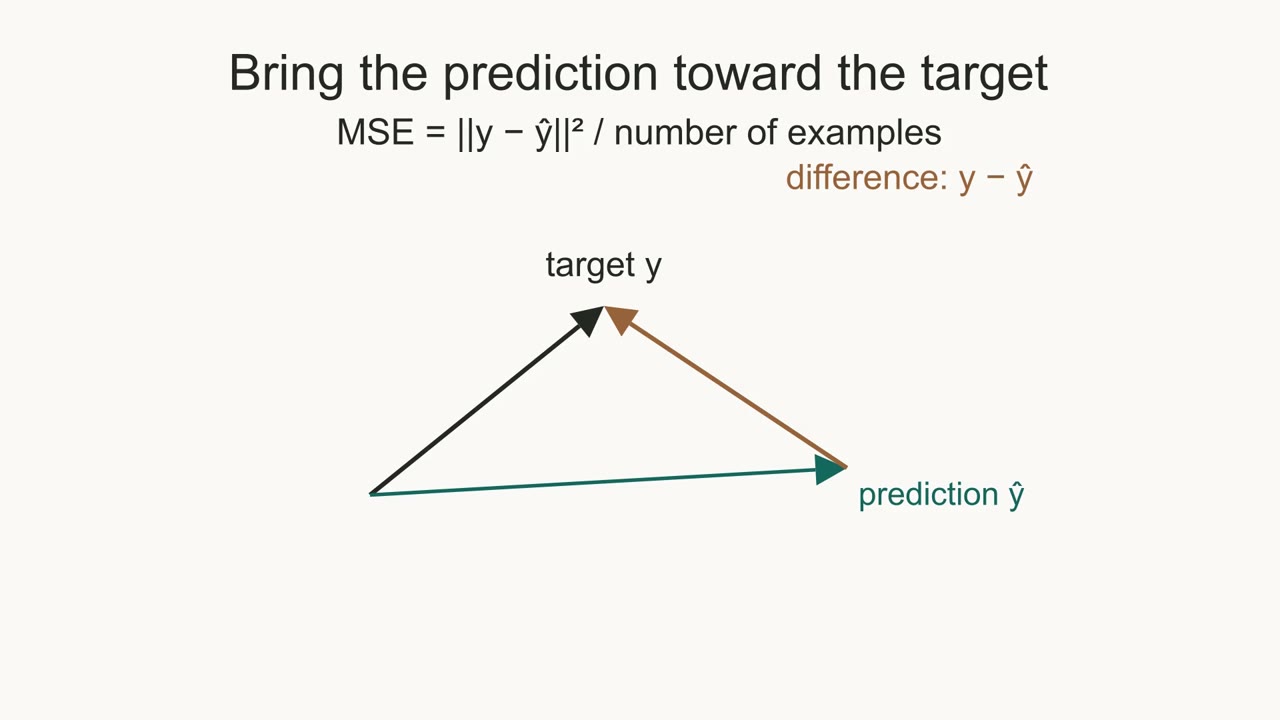
Compare the prediction arrow with the target arrow

The targets form another vector, $y$. The difference $y-\hat y$ is the residual vector. Its coordinates record the prediction errors, including their signs.

Suppose $y=(1,3)$ and $\hat y=(2,1)$. The residual is $(-1,2)$. Squaring and adding gives $(-1)^2+2^2=5$. Average across the two observations:

This is mean squared error. Geometrically, it is the squared distance between the prediction and target vectors, divided by the number of observations. Perfect predictions make the arrows coincide and the residual zero.

Learning changes the weights

Changing $w$ moves $Xw$ within the column space of $X$. Training searches for weights that reduce the loss. Gradient descent takes a small step opposite the loss gradient:

Backpropagation computes gradients through a network; an optimizer uses them to update parameters. Lower training loss measures a better fit to the training examples. Performance on new examples needs its own evaluation.

Read a prediction correctly

Is a raw entry of $Xw$ necessarily a probability?

Answer: No. It is a real-valued score. A probability model needs an appropriate output mapping and training objective.